Mathematics for Machine Learning

Norm

A norm of a vector is a scalar value that defines the magnitude or length of the vector in a vector space. The norm of a vector is useful for various mathematical operations, such as determining the distance between two vectors and defining a metric space. ||x|| determines the norm of the vector.

Different Types of Norms

1. Euclidean norm (also known as the L2 norm):

The Euclidean norm of a vector x = (x1, x2, ..., xn) is defined as:

||x||2 = sqrt(x1^2 + x2^2 + ... + xn^2)

Manhattan norm (also known as the L1 norm):

The Manhattan norm of a vector x = (x1, x2, ..., xn) is defined as:

||x||1 = |x1| + |x2| + ... + |xn|

Max norm (also known as the L-infinity norm):

The Max norm of a vector x = (x1, x2, ..., xn) is defined as:

||x||∞ = max(|x1|, |x2|, ..., |xn|)

Note that ||x|| represents the norm of the vector x.

Dot Product

The dot product, also known as the scalar product or inner product, is a mathematical operation that takes two vectors as input and returns a scalar value. The dot product of two vectors u and v is defined as:

u · v = ||u|| ||v|| cos(θ),

where ||u|| and ||v|| are the magnitudes of the vectors u and v, respectively, and θ is the angle between the two vectors.

Alternatively, the dot product can be defined as:

u · v = sum(u[i] * v[i]) for i = 1 to n,

where n is the number of elements in the vectors u and v.

The dot product has several important properties and applications in mathematics and computer science, including determining the angle between two vectors, projecting one vector onto another, and calculating the work done by a force vector in a certain direction.

Symmetric, Positive Definite Matrix

A symmetric matrix is a square matrix that is equal to its transpose. That is, if A is a symmetric matrix, then A^T = A, where A^T represents the transposition of the matrix A.

A positive definite matrix is a symmetric matrix where the dot product of any non-zero vector with itself, as represented by the matrix, is positive. That is, for any non-zero vector x, the value of x^T A x is positive, where x^T represents the transposition of the vector x.

This code creates a 2x2 symmetric matrix A, which is a simple example of a positive definite matrix. The np.allclose function is used to check if the matrix is symmetric, and the np.linalg.eig function is used to calculate the eigenvalues of the matrix. The np.all function is then used to check if all of the eigenvalues are positive, which indicates that the matrix is positive definite.

import numpy as np

# create a symmetric matrix
A = np.array([[2, 1], [1, 2]])

# check if the matrix is symmetric
print("Symmetric: ", np.allclose(A, A.T))

# calculate eigenvalues
eigenvalues, _ = np.linalg.eig(A)

# check if all eigenvalues are positive
print("Positive definite: ", np.all(eigenvalues > 0))
#Symmetric:  True
#Positive definite:  True

Distance between vector

The norms discussed above can also be used to calculate the distance between vectors. Cosine similarity is a measure of similarity between two non-zero vectors of an inner product space. It is defined as:

similarity = (u · v) / (||u|| ||v||)

import numpy as np

def euclidean_distance(u, v):
    return np.linalg.norm(u - v)


def manhattan_distance(u, v):
    return np.sum(np.abs(u - v))

def cosine_similarity(u, v):
    dot_product = np.dot(u, v)
    magnitude_u = np.linalg.norm(u)
    magnitude_v = np.linalg.norm(v)
    return dot_product / (magnitude_u * magnitude_v)

The angle between vectors and orthogonality

The angle between two vectors in a Euclidean space is a measure of the orientation of the vectors relative to each other. It can be calculated using the dot product and the magnitudes of the vectors.

The cosine of the angle between two non-zero vectors u and v can be calculated as:

cos(θ) = (u · v) / (||u|| ||v||),

where u · v is the dot product of the vectors u and v, and ||u|| and ||v|| are the magnitudes of the vectors u and v, respectively.

Orthogonality is a concept in linear algebra that refers to the property of two vectors being perpendicular, or having an angle of 90 degrees, in a Euclidean space. Two vectors u and v are orthogonal if and only if their dot product is zero:

u · v = 0

Orthogonal Matrix

An orthogonal matrix is a square matrix whose columns and rows are orthogonal unit vectors. This means that the dot product of any two distinct columns or rows is equal to zero, and the magnitude of each column or row is equal to 1.

An orthogonal matrix Q has the following properties:

QTQ = QQT = I, where QT is the transposition of Q and I is the identity matrix.
The determinant of Q is either 1 or -1.

In linear algebra, orthogonal matrices are used to represent rotations and reflections in a Euclidean space. An orthogonal matrix Q can be used to rotate a vector x by multiplying Qx, and the resulting vector will be a rotation of the original vector. The transposition of an orthogonal matrix is also an orthogonal matrix and represents the inverse transformation.

Inner Product of the Function

In mathematics, an inner product of a function is a mathematical operation that takes two functions as input and produces a scalar as output. It is a generalization of the dot product of two vectors in Euclidean space.

Given two functions f(x) and g(x) defined on a certain domain, their inner product is defined as: ⟨f, g⟩ = ∫ f(x)g(x) dx

Orthogonal Functions

Two functions are said to be orthogonal if their inner product is zero.

Formally, two functions f(x) and g(x) are said to be orthogonal on a given interval [a,b] if their inner product over that interval is zero, i.e., if:

`∫a to b f(x)g(x) dx = 0`

It's worth noting that the notion of orthogonality is closely related to the concept of independence, as orthogonal functions are also linearly independent, which means that neither of them can be expressed as a linear combination of the other.

Some examples of orthogonal functions include the Legendre polynomials, the Chebyshev polynomials, and the trigonometric functions sine and cosine over the interval [-π,π]. Orthogonal functions are useful in many areas of mathematics and science because they provide a way to decompose more complex functions into simpler, orthogonal components, which can be easier to analyze and understand.

Legendre polynomials

The Legendre polynomials are defined recursively by the formula:

P_0(x) = 1 P_1(x) = x (n+1)P_{n+1}(x) = (2n+1)xP_n(x) - nP_{n-1}(x)

where n is a non-negative integer, and P_n(x) denotes the nth Legendre polynomial.

The first few Legendre polynomials are:

P_0(x) = 1

P_1(x) = x

P_2(x) = (3x^2 - 1)/2

P_3(x) = (5x^3 - 3x)/2

P_4(x) = (35x^4 - 30x^2 + 3)/8

Chebyshev Polynomials

The Chebyshev polynomials are a family of orthogonal polynomials that arise in many areas of mathematics, such as approximation theory, numerical analysis, and signal processing.

The Chebyshev polynomials of the first kind, denoted T_n(x), are defined by the recurrence relation:

T_0(x) = 1 T_1(x) = x T_{n+1}(x) = 2xT_n(x) - T_{n-1}(x)

The first few Chebyshev polynomials of the first kind are:

T_0(x) = 1 T_1(x) = x T_2(x) = 2x^2 - 1 T_3(x) = 4x^3 - 3x T_4(x) = 8x^4 - 8x^2 + 1

The Legendre, Chebyshev polynomials have several important properties, including orthogonality, which means that the integral of the product of any two Legendre polynomials over the interval [-1,1] is zero unless they are the same polynomial. This property makes them useful in approximating functions over the interval [-1,1], and in solving differential equations, among other applications.

Projection

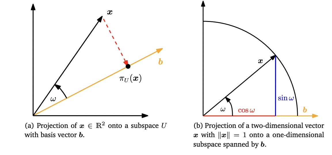
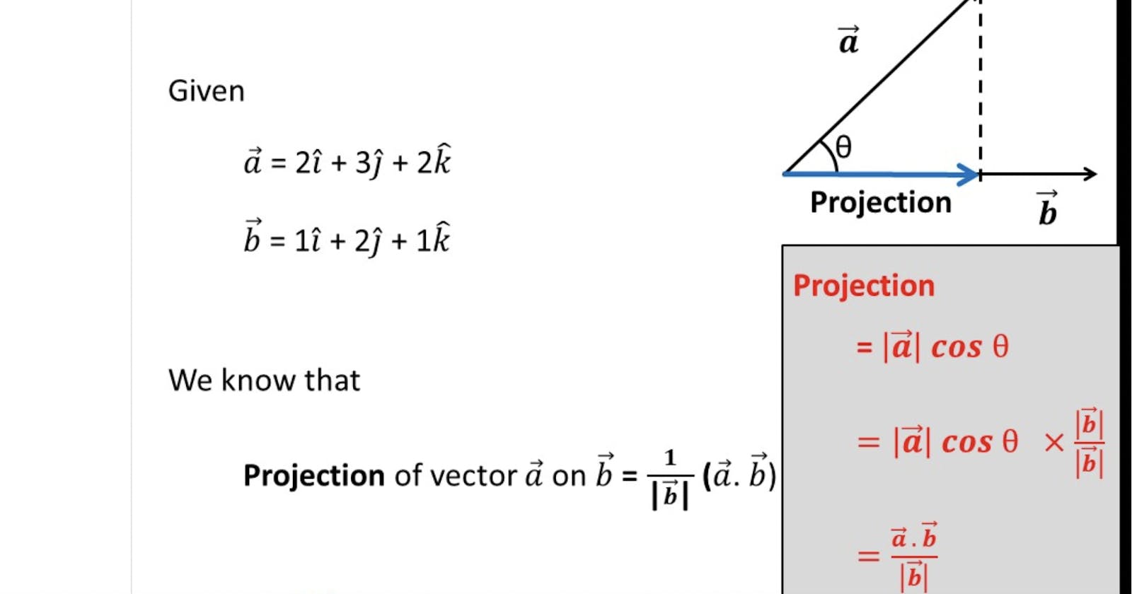
A projection refers to the process of projecting a vector onto a subspace. Given a vector space V and a subspace U of V, the projection of a vector v in V onto U is a vector that lies in U and is closest to v.

More specifically, if we let u1, u2, ..., um be an orthogonal basis for U, then the projection of v onto U is given by the formula:

projU(v) = ((v · u1)/||u1||^2) u1 + ((v · u2)/||u2||^2) u2 + ... + ((v · um)/||um||^2) um,

where · denotes the dot product and || || denotes the norm.

Taken from Mathematics for Machine Learning Book

https://www.youtube.com/watch?v=27vT-NWuw0M&t=10s&ab_channel=KhanAcademy

Below is Python code to project a vector b xy plane and z axis:

import numpy as np

P_z = np.matrix([[0, 0, 0], [0, 0, 0], [0, 0, 1]])
P_xy = np.matrix([[1, 0, 0], [0, 1, 0], [0, 0, 0]]) 

b = np.matrix([2,9,5])
p_xy = P_xy*b.T
p_z = P_z*b.T

print("projection of b on xy space", p_xy)
print("projection of b on z axis", p_z)

##projection of b on xy space 
#[[2]
#[9]
#[0]]
##projection of b on z axis 
#[[0]
#[0]
#[5]]
##

Span of the Vector

The span of a vector or a set of vectors is the set of all possible linear combinations of those vectors. In other words, it is the set of all vectors that can be expressed as a linear combination of the original vectors.

For example, consider two vectors in R2:

u = [1, 2] v = [3, 4]

The span of these vectors is the set of all possible linear combinations of u and v:

span{u, v} = {au + bv | a, b ∈ R}

where au + bv is a linear combination of u and v.

In this case, the span of {u, v} is the entire plane R2, since any point in R2 can be expressed as a linear combination of u and v.