Vector Space

A group is a mathematical structure consisting of a set of elements and a binary operation that takes two elements and returns a third element in the set. The operation must satisfy four properties:

1. Closure: The result of the operation is always in the set. ⊗: ∀x, y ∈ G : x ⊗ y ∈ G

2. Associativity: The order in which the operation is performed does not affect the result. ∀x, y, z ∈ G : (x ⊗ y) ⊗ z = x ⊗ (y ⊗ z)

3. Identity element: There is an element in the set such that when it is operated on with any other element, the other element is unchanged. ∃e ∈ G ∀x ∈ G : x ⊗ e = x and e ⊗ x = x

4. Inverse element: For every element in the set, there exists another element in the set such that when the two elements are operated on, the identity element is obtained. ∀x ∈ G ∃y ∈ G : x ⊗ y = e and y ⊗ x = e

Vector spaces have few additional properties beyond groups for scalars.

1. Vectors can be scaled by multiplying them with scalars.

2. Scalar Addition is Distributive

3. Scalar multiplicationn is Associative.

4. Multiplying the vector by 1 keeps it unchanged.

Vector Subspace

A vector subspace is a subset of a vector space that is itself a vector space with the same operations. This means that if a set of vectors is a subspace, then it must also satisfy all of the properties of a vector space, including closure under addition and scalar multiplication, the existence of a zero vector, and so on.

Formally, a non-empty subset V of a vector space W is a vector subspace if and only if it satisfies the following two conditions:

1. Closure under addition: For any two vectors u and v in V, their sum u + v is also in V.

2. Closure under scalar multiplication: For any scalar c and any vector u in V, the product c.u is also in V.

The zero vector of the subspace is the same as the zero vector of the original vector space, and the additive inverse of a vector in the subspace is also a vector in the subspace.

We are going to slightly deviate from LA to probability and discuss Chi-square test:

https://www.youtube.com/watch?v=2QeDRsxSF9M

Chi-Square Test (Goodness of Fit)

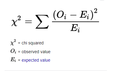
The chi-square test is a statistical test used to determine whether there is a significant difference between the expected and observed frequencies in one or more categorical variables. The test is used to analyze the relationship between two categorical variables by comparing the observed data to the expected data under the null hypothesis of independence between the variables.

Chi-square Test is used for:

1. Feature selection: In classification problems, the chi-square test can be used to select the most informative features for the classification task. By calculating the chi-square statistic for each feature and the target variable, we can identify the features that are most correlated with the target variable and select them for the model.

2. Goodness of fit testing: The chi-square test can be used to test the goodness of fit of a model to the data. By comparing the observed frequencies to the expected frequencies predicted by the model, we can determine if the model is a good fit for the data.

SelectKBest method for Feature Selection

SelectKBest is a feature selection method in machine learning that selects the k most informative features from a dataset. The selection is based on univariate statistical tests, where each feature is evaluated independently in terms of its correlation with the target variable. The k best features are selected based on their scores, which are typically derived from a statistical test such as the chi-square test or the F-test.

SelectKBest is commonly used to reduce the dimensionality of a dataset, which can improve the performance of a model and reduce overfitting. By selecting only the most informative features, we can simplify the model and remove noise or irrelevant features.

Let's write a Python code, that applies vector subspace for feature selection. Below code loads, the Iris dataset converts the data to a Pandas DataFrame and then applies the SelectKBest method with the chi2 scoring function to select the top 2 features. The names of the selected features are then printed. In this example, the SelectKBest the method performs a chi-squared test to score each feature based on its relationship with the target variable, and the top 2 features are selected. You can change the value of k to select a different number of features. We would discuss in detail about code in upcoming articles.

import numpy as np
import pandas as pd
from sklearn.datasets import load_iris
from sklearn.feature_selection import SelectKBest, chi2

# Load the Iris dataset
iris = load_iris()
X = iris.data
y = iris.target

# Convert the data to a Pandas DataFrame for easy analysis
df = pd.DataFrame(X, columns=iris.feature_names)

# Select the top 2 features using chi-squared test
selector = SelectKBest(chi2, k=2)
X_new = selector.fit_transform(X, y)

# Get the names of the selected features
selected_features = df.columns[selector.get_support()]
print("Selected features: ", selected_features)

#Selected features:  Index(['petal length (cm)', 'petal width (cm)'], dtype='object')

Linear Independence

Linear independence of vectors is a concept in linear algebra that refers to the property of a set of vectors where no vector in the set can be expressed as a linear combination of the others.

Formally, a set of vectors {v1, v2, ..., vn} in a vector space is said to be linearly independent if and only if the only solution to the equation:

a1v1 + a2v2 + ... + an * vn = 0

where a1, a2, ..., an are scalars, is a1 = a2 = ... = an = 0. In other words, the only way to get a zero vector by combining the vectors in the set is to use the scalar 0.

Linear independence is used in several ways in machine learning:

1. Overfitting: In linear regression and other linear models, having too many features can lead to overfitting. By using a feature selection algorithm that chooses linearly independent features, it's possible to reduce the number of features and reduce the risk of overfitting.

2. Feature Engineering: When designing new features for a machine learning model, it's often a good idea to choose linearly independent features. This ensures that the features provide unique information about the data and are not redundant.

3. Eigenvectors: Eigenvectors are linearly independent vectors that are used to represent the data in a new, lower-dimensional space.

4. Orthogonal Projection: Orthogonal projection is a technique used in linear regression and other linear models to project the data onto a subspace spanned by linearly independent vectors. This can be used to reduce the dimensionality of the data and improve the interpretability of the model.

5. Regularization: Regularization is a technique used in linear models to prevent overfitting by adding a penalty term to the loss function that discourages the model from fitting the training data too well. One type of regularization, ridge regression, uses a linear combination of linearly independent features.

import numpy as np
import matplotlib.pyplot as plt
from sklearn.linear_model import LinearRegression

# Generate toy data
np.random.seed(0)
x = np.sort(5 * np.random.rand(80, 1), axis=0)
y = np.sin(x).ravel()
y[::5] += 3 * (0.5 - np.random.rand(16))

# Split the data into training and test sets
x_train, x_test = x[:60], x[60:]
y_train, y_test = y[:60], y[60:]

# Fit a linear regression model to the training data
reg = LinearRegression().fit(x_train, y_train)

# Predict the outputs on the training and test data
y_train_pred = reg.predict(x_train)
y_test_pred = reg.predict(x_test)

# Plot the data and the predictions
plt.scatter(x_train, y_train, color='red', label='Training data')
plt.scatter(x_test, y_test, color='blue', label='Test data')
plt.plot(x_train, y_train_pred, color='black', label='Training prediction')
plt.plot(x_test, y_test_pred, color='green', label='Test prediction')
plt.legend()
plt.show()

You can see that the model fits the training data well, but it overfits the data, as the prediction on the test data is not as good as the prediction on the training data.

Basis Vector

Basis vectors are a set of mutually orthogonal (perpendicular) vectors used to represent any vector in a given vector space. In a space of N dimensions, N basis vectors are used to represent any vector in that space as a linear combination of the basis vectors.

In 3-dimensional Euclidean space, the standard basis vectors are often represented using unit vectors along the x, y, and z-axis, denoted as î, ĵ, and k̂ respectively. These vectors have a magnitude of 1 and are orthogonal to each other, meaning they are at 90 degrees to each other.

For example, vector (3,4,5) can be represented as 3î + 4 ĵ + 5k̂ = (3,4,5). This means that this vector is 3 units along the x-axis (î), 4 units along the y-axis (ĵ), and 5 units along the z-axis (k̂).

Homomorphism and Linear Transformation

A homomorphism is a mathematical function between two algebraic structures that preserves the operations of the structures. In other words, a homomorphism maps elements of one structure to elements of another structure in such a way that the operations of the two structures are preserved.

A linear transformation is a kind of Homomorphism that transforms one vector space into another vector space, preserving the properties of vector addition and scalar multiplication.

Mathematically, a linear transformation can be represented as a matrix, where the transformation of a vector can be found by matrix-vector multiplication. The matrix represents how the basis vectors of the input space are transformed into the basis vectors of the output space. The properties of vector addition and scalar multiplication are preserved because the matrix representation is linear, meaning that the transformation of a sum of vectors is equal to the sum of the transformations of individual vectors, and the transformation of a scalar multiple of a vector is equal to the scalar multiple of the transformation of the vector.

Let's do a Linear Transformation for a vector that changes the basis of the vector. In this example, the original basis vectors are stored in basis_A and the new basis vectors are stored in basis_B. The matrix P represents the change of basis from basis_A to basis_B, and is obtained by multiplying basis_B by the inverse of basis_A. Finally, the vector x is transformed into a new basis by multiplying it by P. The resulting vector y represents the original vector x in the new basis.

import numpy as np

# Define the original basis vectors
basis_A = np.array([[1, 0], [0, 1]])

# Define the new basis vectors
basis_B = np.array([[1, 1], [1, -1]])

# Define the matrix representing the change of basis from basis_A to basis_B
P = np.dot(basis_B, np.linalg.inv(basis_A))

# Define the vector in the original basis
x = np.array([2, 3])

# Perform the change of basis
y = np.dot(P, x)

print("Original vector: ", x)
print("Vector in new basis: ", y)
#Original vector:  [2 3]
#Vector in new basis:  [ 5. -1.]
#

Image and Kernel

Image of linear mapping is the set of all vectors in the target vector space that can be obtained by applying the linear mapping to vectors in the original vector space. It represents the set of all possible outputs of the linear mapping.

Kernel of linear mapping, on the other hand, is the set of all vectors in the original vector space that are mapped to the zero vector in the target vector space. It represents the set of inputs for which the linear mapping has no effect.

The image and kernel of a linear mapping can be used to study the properties of the mapping and to understand its behaviour. For example, the dimension of the image can give information about how much the mapping changes the vectors, while the dimension of the kernel can give information about the number of degrees of freedom or the number of independent inputs that the mapping can accept.

In this example, the matrix A represents linear mapping. The range function from the Numpy linear algebra library is used to find the image of the linear mapping, which is stored in the variable image. The null function is used to find the kernel of the linear mapping, which is stored in the variable kernel.

import numpy as np

# Define the matrix representing the linear mapping
A = np.array([[1, 2], [3, 4]])

# Find the image of the linear mapping
image = np.linalg.range(A)
print("Image: ", image)

# Find the kernel of the linear mapping
kernel = np.linalg.null(A)
print("Kernel: ", kernel)
#Image:  [0 1 2 3]
#Kernel:  [[-2.]
 #        [ 1.]]

References:

https://mml-book.github.io/book/mml-book.pdf

https://www.youtube.com/watch?v=ozwodzD5bJM&ab_channel=Socratica

https://textbooks.math.gatech.edu/ila/linear-transformations.html